


Feature Engineering for Predicting Poverty
Introduction
We recently competed in the machine learning Kaggle competition, Costa Rican Household Poverty Level Prediction, placing 15th out of 619 participants (top 3%). This competition involved predicting a classification of poverty for a household (extreme poverty, moderate poverty, vulnerable household, or non-vulnerable household) based on information from a household-level survey. Similar to many of the other solutions submitted, we used a gradient boosted framework, LightGBM. Although setting up the model and conducting hyper-parameter tuning posed many challenges, this blog post focuses on what we thought were two interesting feature engineering techniques. These techniques lead to features that had high predictive performance within the model.
Background
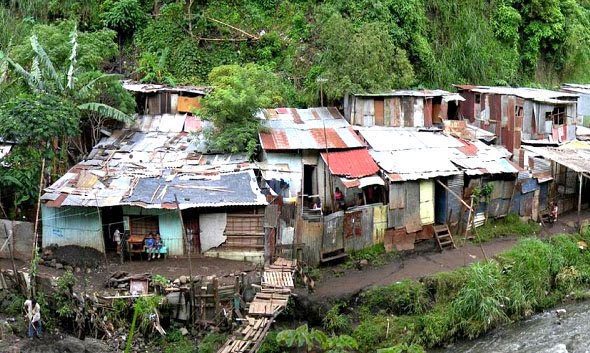
There are many aspects to poverty which go beyond monetary considerations. Poverty can include lack of available resources such as education, health care, security, and clean water. However, when we measure poverty it is generally from a monetary perspective. There are several ways to measure poverty, in an absolute sense or in a relative sense. Both methods use a poverty line to categorize households (above or below the poverty line) but they differ in how they construct the poverty line. In an absolute sense, the poverty line is defined by the minimum amount of income to maintain a basic standard of living including food, clothing, and shelter. In a relative sense, the poverty line can be defined as a certain percentage of the median household income. Both of these methods require either directly measuring a household’s income or some proxy of that income. Direct measurement of household income is difficult due to factors such as poor record keeping and the importance of secondary capital sources such as self-produced goods and food, gifts, and remittances. Because of these difficulties, social aid programs often choose to measure and classify poverty by measuring proxies for income. This can include things such as asset ownership, including mobile phone, television, or laptop computer. In addition, proxies can be related to household characteristics such as, roof, wall, and ceiling material type, the presence of running water, the presence of electricity, or number of bedrooms. These types of proxies are easily observable and verifiable by the survey collector, leading to more accurate data collection.
Proxy means testing (PMT) is a method to relate a poverty classification to various household proxies and has been adopted by many countries as the method for selecting beneficiaries for social aid programs. The advantage of this method is the reliability of the underlying data and the ease of collection. Usually, PMT is modeled using an ordinary least squares (OLS) regression to relate household characteristics to income. The goal of this Kaggle competition was to see if there are other methods to determine household poverty classifications which might perform better than traditional linear regressions.
Feature Engineering
Feature engineering is the process of applying specific domain knowledge to create new features (or model inputs) which help a model make correct predictions. In a sense, this is formulating the correct questions for a model to ask so that it may successfully predict an outcome. Although there are several steps in successfully setting up and solving a machine learning problem we focus on feature engineering because it’s a crucial step for the success of a model.
Many real world problems involve the response variable as a complex function of the features or inputs of a model. When the raw inputs are not in a form which allows easy learning for the model, your ability to predict the response variable will be limited. This was definitely the case for the Kaggle competition predicting household poverty.
Engineering features involves specific domain knowledge of the problem at hand. Our previous experience in international development help guide the methods we used to develop new features. Below we present two methods of feature engineering we used for this particular Kaggle competition which helped boost our model performance.
Multiple Correspondence Analysis (MCA)
The Costa Rican household survey (Kaggle data set) contained a whole slew of questions related to asset ownership and household characteristics. For asset ownership, the survey included questions regarding ownership of home, tablets, and mobile phones. For household characteristics, the survey included questions related to the number of bedrooms, presence of electricity, presence of toilet, and material and condition of walls, roof, and floor. The idea behind asset ownership and household characteristic questions is that wealthier families will own more assets and their homes will be in better conditions and have more amenities than poorer families. The difficulty lies in the fact that the classification of wealth of the household is spread across many inputs. We would like represent the economic status of a household as proxied by asset ownership and household characteristics with only one or two variables.
Reducing the dimensionality of inputs allows us to reduce the amount of features used in the model while still retaining the important information regarding wealth classification as described by the the full set of asset ownership and household characteristic questions. The dimensionality reduction can lead to better predictive performance in machine learning models because you are potentially removing extraneous noise from the system.
One possible method for reducing dimensionality of asset ownership data is Principal Component Analysis (PCA) (Filmer and Pritchett, 1998; Córdova, A., 2009). Household assets and characteristics often have overlap. For example, if a household has bathroom facilities within the structure, they most likely have running water. PCA allows one to best describe the assets and characteristics of the household with a new reduced number of values.
For this Kaggle competition, the majority of variables that describe household assets or characteristics are categorical variables. For example, either binary (Yes/No) or classification (such as building material type). We could have apply the tradition PCA analysis to this dataset; however, we believe that economic status of the household is best represented by the relative combination of the categorical variables related to asset ownership and household characteristics. Therefore we chose to utilize Multiple Correspondence Analysis (MCA). Further description of MCA can be found in Nenadic and Greenacre, 2005. The calculated principal components from MCA are new features that best summarize the relative combinations of the household assets and characteristic variables.
The Kaggle competition had many categorical variables which represent the household’s assets and characteristics. The table below shows a subset of the variables we chose:
| Variable | Description | Type |
|---|---|---|
| V18q | Owns a tablet computer | Binary (Yes/No) |
| computer | Household has a desktop or laptop computer |
Binary (Yes/No) |
| television | Household has a television | Binary (Yes/No) |
| mobile | Household has a mobile phone | Binary (Yes/No) |
| tipovivi | Classification of house ownership |
- House is owned and fully paid for - House is owned and paying installments -House is rented -Precarious -Other |
| v14a | Has a toilet in household | Binary (Yes/No) |
| refrig | Has a refrigerator | Binary (Yes/No) |
| paredblolad | Classification of predominant material of outside wall of house |
Block or brick, Prefabrication or cement, Waste material, etc. |
| piso | Classification of predominate material of floor |
Ceramic, Cement, Wood, etc. |
| techo | Classification of predominate material of roof |
Wood, Metal, Fiber cement, etc. |
| cielorazo | House has a roof | Binary (Yes/No) |
| abastagua | Classification of water provision | -Water provision inside the house -Water provision outside the house -No water provision |
| elec | Classification of source of household electricity |
-Electricity from private plant -Electricity from cooperative -No electricity from dwelling |
To calculate the principal components of MCA on these categorical variables we used the Python Prince (Python factor analysis library) library. This library makes calculating the MCA simple with a few lines of code:
from prince import MCA


mca = MCA(n_components=2)
hh_assests_mca = mca.fit_transform(x_vars)

# Extract the first component
mca_1 = hh_assests_mca[0]

# Extract the second component
mca_2 = hh_assests_mca[1]
Although in the competition we used the first 3 principal components from the MCA, below we plot two principal components (x and y axis) for each household colored by their corresponding poverty classification. These components are directly used as features in the gradient boosted model for classification of poverty.
Geospatial Aggregation
In addition to considering the asset ownership and physical characteristics of a household, it is important to consider the role of geography in social economic status. Throughout the world, regardless of a country’s economic stature, standards of living between regions and communities can vary significantly. These variations are often too significant to be explained by differences in households assets or characteristics. In developing countries, the geographic disparities in living standards persist because of obstacles to internal migration (Bigman and Fofack, 2000). Therefore, when comparing measures of wealth it’s important to put these in a region or community context. Fortunately, the Kaggle dataset had information for each household about the region that household resides in.
If we assume, in the Kaggle competition data set, that the sample of households for each region is representative of the population of those regions we can compare the distribution of household poverty classification across regions. The figure below shows the fraction of total households which fall into each poverty classification broken down by region. The y-axis is the fraction of total households (by region) and the x-axis is the poverty classification. The various colors represent separate regions.

The figure clearly shows that households in region 3 (green) are more likely to be vulnerable or in a state of poverty versus other regions. Region 3 has the lowest fraction of households which exist in the non-vulnerable group. Households in Region 1 (blue) are more likely to be non-vulnerable. This region has the highest fraction of total households in the non-vulnerable classification.
Again, it’s important to understand the context of the household survey and to make sure that the survey was conducted in such a manner that the sample of households for each region is representative of the total population of that region. If this is not the case, it is possible that the difference in distribution is an artifact of survey sampling and not a representation of difference due to geography.
Assuming that we have a representative sample, the above figure shows that it’s important to consider geographic information when making a prediction. One straightforward way to do this is to include region as an explanatory variable or feature. Another way is to construct z-scores of various features based on the regional specific distribution of the parameters. The z-score allows us to view the household specific value for a feature in terms of the distribution of that feature in a region. Is it close to the mean value or is it significantly above or below the mean value? This grounds the feature to the distribution for a specific region. The mean values of features may hold different weights in predicting poverty classification for different regions.
Utilizing the Pandas library in Python calculating these region specific z-scores is relatively straight forward:
# Using Pandas Dataframe method groupby we calculate the mean values of features for each region
region_aggs_mean = df_total.groupby('enc_lugar').mean().reset_index()

# Extract a list of column names excluding the region column
mean_cols = [str(col) for col in region_aggs_mean.columns if col != 'enc_lugar']

# Rename columns indicating they are mean values
region_aggs_mean.rename(columns=dict((k, "loc_mean_" + k) for k in mean_cols), inplace=True)

# Using Pandas Dataframe method groupby we calculate the standard deviation of features for each region
region_aggs_std = df_total.groupby('enc_lugar').std().reset_index()

# Extract a list of column names excluding the region column
std_cols = [str(col) for col in region_aggs_std.columns if col != 'enc_lugar']

# Rename columns indicating they are mean values
region_aggs_std.rename(columns=dict((k, "loc_std_" + k) for k in std_cols), inplace=True)

# Merge the calculated means and std back into the original dataframe
df = df.merge(region_aggs_mean, on='enc_lugar', how='left')
df = df.merge(region_aggs_std, on='enc_lugar', how='left')

# For a specific list of features (geo_var) calculate the regional based z-score
for gc in geo_vars:
    df[gc + '_zscore'] = (df['loc_mean_' + gc] - df[gc]) / df['loc_std_' + gc]
Summary
We hope you have enjoyed this blog post on feature engineering techniques we used for predicting poverty classification from Costa Rica household survey data. We presented two different methodologies to engineer new features which then go into a classification model (Gradient Boosted framework in our case). We utilized these methods based on our previous experience in the humanitarian aid sector. At Visual Perspective, we are big fans of machine learning; however, we also recognize the importance of researching and understanding domain specific knowledge of the problem you are trying to solve. Our passion is to create meaningful visualization and understanding of data. Let us know how we can help you, contact us.
Footnote
We should note that one of the features that had significant predictive power and required no engineering was the amount of education of the individuals within the household. Our model showed higher rates of education are related to lower rates of poverty. This aligns with previous thought that education and poverty are related (Patel and Kleinman, 2003; Tilak, 2007). Our observation does not establish causality, in other words, it does not prove that higher education rates cause a decrease in poverty. It could be that households who are not in poverty are able to spend more resources on education. They do not require all members of the household to earn income and therefore they are free to pursue an education. However, it’s worth considering the development of educational programs for the long term solution of eliminating poverty.
References
Bigman, D. and Fofack, H., 2000. Geographical targeting for poverty alleviation: An introduction to the special issue. The World Bank Economic Review, 14(1), pp.129-145.
Clay, D.C., Molla, D. and Habtewold, D., 1999. Food aid targeting in Ethiopia: A study of who needs it and who gets it. Food policy, 24(4), pp.391-409.
Córdova, A., 2009. Methodological note: Measuring relative wealth using household asset indicators. AmericasBarometer Insights, 6, pp.1-9.
Filmer, D. and Pritchett, L., 1998. Estimating Wealth Effects without Expenditure Data--or Tears: An Application to Educational Enrollments in States of India. Policy Research Working Papers No. 1994.
Kidd, S. and Wylde, E., 2011. Targeting the Poorest: An assessment of the proxy means test methodology. AusAid Research Paper, AusAid, Canberra.
Kidd, S., Gelders, B. and Bailey-Athias, D., 2017. Exclusion by design: An assessment of the effectiveness of the proxy means test poverty targeting mechanism. International Labour Organization.
Kirby, M., 2000. Geometric data analysis: an empirical approach to dimensionality reduction and the study of patterns. John Wiley & Sons, Inc.
Nenadic, O. and Greenacre, M., 2005. Computation of multiple correspondence analysis, with code in R.
Patel, V. and Kleinman, A., 2003. Poverty and common mental disorders in developing countries. Bulletin of the World Health Organization, 81, pp.609-615.
Tilak, J.B., 2007. Post-elementary education, poverty and development in India. International Journal of Educational Development, 27(4), pp.435-445.